Automatically identifying voicemails
Back in 2015, prosecutor Alberto Nisman was found dead under suspicious circumstances, just as he was about to bring a complaint accusing the Argentinian President Fernández over interfering with investigations into the AMIA bombing that took place in 1994 (This Guardian piece provides some good background).
There were some 40,000 phone calls related to the case that La Nación was interested in exploring further. Naturally, that is quite a big number and it’s hard to gather the resources to comb through that many hours of audio.
La Nación crowdsourced the labeling of about 20,000 of these calls into those that were interesting and those that were not (e.g. voicemails or bits of idle chatter). For this process they used CrowData, a platform built by Manuel Aristarán and Gabriela Rodriguez, two former Knight-Mozilla Fellows at La Nación. This left about 20,000 unlabeled calls.
While Juan and I were in Buenos Aires for the Buenos Aires Media Party and our OpenNews fellows gathering, we took a shot at automatically labeling these calls.
Data preprocessing
The original data we had was in the form of mp3s and png images produced from the mp3s. wav files are easier to work with so we used ffmpeg to convert the mp3s. With wav files, it is just a matter of using scipy to load them as numpy arrays.
For instance:
from scipy.io import wavfile

sample_rate, data = wavfile.read('/path/to/file.wav')
print(data)
# [15,2,5,6,170,162,551,8487,1247,15827,...]
In the end however, we used librosa, which normalizes the amplitudes and computes a sample rate for the wav file, making the data easier to work with.
import librosa

data, sr = librosa.load('/path/to/file.wav', sr=None)
print(data)
# [0.1,0.3,0.46,0.89,...]
These arrays can be very large depending on the audio file’s sample rate, and quite noisy too, especially when trying to identify silences. There may be short spikes in amplitude in an otherwise “silent” section, and in general, there is no true silence. Most silences are just low amplitude but not exactly 0.
In the example below you can see that what a person might consider silence has a few bits of very quiet sound scattered throughout.
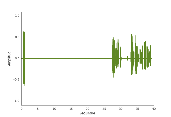
There is also “noise” in the non-silent parts; that is, the signal can fluctuate quite suddenly, which can make analysis unwieldy.
To address these concerns, our preprocessing mostly consisted of:
- Reducing the sample rate a bit so the arrays weren’t so large, since the features we looked at don’t need the precision of a higher sample rate.
- Applying a smoothing function to deal with intermittent spikes in amplitude.
- Zeroing out any amplitudes below 0.015 (i.e. we considered any amplitude under 0.015 to be silence).
Since we had about 20,000 labeled examples to process, we used joblib to parallelize the process, which improved speeds considerably.
The preprocessing scripts are available here.
Feature engineering
Typically, the main challenge in a machine learning problem is that of feature engineering - how do we take the raw audio data and represent it in a way that best suits the learning algorithm?
Audio files can be easily visualized, so our approach benefited from our own visual systems - we looked at a few examples from the voicemail and non-voicemail groups to see if any patterns jumped out immediately. Perhaps the clearest two patterns were the rings and the silence:
- A voicemail file will also have a greater proportion of silence than sound. For this, we looked at the images generated from the audio and calculated the percentage of white pixels (representing silence) in the image.
- A voicemail file will have several distinct rings, and the end of the file comes soon after the last ring. The intuition here is that no one picks up during a voicemail - hence many rings - and no one stays on the line much longer after the phone stops ringing. So we consider both the number of rings and the time from the last ring to the end of the file.
Ring analysis
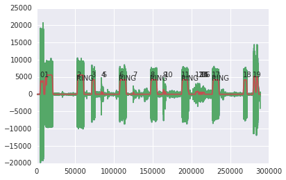
Identifying the rings is a challenge in itself - we developed a few heuristics which seem to work fairly well. You can see our complete analysis here, but the general idea is that we:
- Identify non-silent parts, separated by silences
- Check the length of the silence that precedes the non-silent part, if it is too short or too long, it is not a ring
- Check the difference between maximum and minimum amplitudes of the non-silent part; it should be small if it’s a ring
The example below shows the original audio waveform in green and the smoothed one in red. You can see that the rings are preceded by silences of a roughly equivalent length and that they look more like plateaus (flat-ish on the top). Another way of saying this is that rings have low variance in their amplitude. In contrast, the non-ring signal towards the end has much sharper peaks and vary a lot more in amplitude.
Other features
We also considered a few other features:
- Variance: voicemails have greater variance, since there is lots of silence punctuated by high-amplitude rings and not much in between.
- Length: voicemails tend to be shorter since people hang up after a few rings.
- Max amplitude: under the assumption that human speech is louder than the rings
- Mean silence length: under the assumption that when people talk, there are only short silences (if any)
However, after some experimentation, the proportion of silence and the ring-based features performed the best.
Selecting, training, and evaluating the model
With the features in hand, the rest of the task is straightforward: it is a simple binary classification problem. An audio file is either a voicemail or not. We had several models to choose from; we tried logistic regression, random forest, and support vector machines since they are well-worn approaches that tend to perform well.
We first scaled the training data and then the testing data in the same way and computed cross validation scores for each model:
LogisticRegression
    roc_auc: 0.96 (+/- 0.02)
    average_precision: 0.94 (+/- 0.03)
    recall: 0.90 (+/- 0.04)
    f1: 0.88 (+/- 0.03)
RandomForestClassifier
    roc_auc: 0.96 (+/- 0.02)
    average_precision: 0.95 (+/- 0.02)
    recall: 0.89 (+/- 0.04)
    f1: 0.90 (+/- 0.03)
SVC
    roc_auc: 0.96 (+/- 0.02)
    average_precision: 0.94 (+/- 0.03)
    recall: 0.91 (+/- 0.04)
    f1: 0.90 (+/- 0.02)
We were curious what features were good predictors, so we looked at the relative importances of the features for both logistic regression:
[('length', -3.814302896584862),
 ('last_ring_to_end', 0.0056240364270560934),
('percent_silence', -0.67390678402142834),
('ring_count', 0.48483923341906693),
('white_proportion', 2.3131580570928114)]
And for the random forest classifier:
[('length', 0.30593363755717351),
 ('last_ring_to_end', 0.33353202776482688),
 ('percent_silence', 0.15206534339705702),
 ('ring_count', 0.0086084243372190443),
 ('white_proportion', 0.19986056694372359)]
Each of the models perform about the same, so we combined them all with a bagging approach (though in the notebook above we forgot to train each model on a different training subset, which may have helped performance), where we selected the label with the majority vote from the models.
Classification
We tried two variations on classifying the audio files, differing in where we set the probability cutoff for classifying a file as uninteresting or not.
in the balanced classification, we set the probability threshold to 0.5, so any audio file that has ≥ 0.5 of being uninteresting is classified as uninteresting. This approach labeled 8,069 files as discardable. in the unbalanced classification, we set the threshold to the much stricter 0.9, so an audio file must have ≥ 0.9 chance of being uninteresting to be discarded. This approach labeled 5,785 files as discardable.
You can see the Jupyter notebook where we conducted the classification here.
Validation
We have also created a validation Jupyter notebook where we can cherry pick random results from our classified test set and verify the correctness ourselves by listening to the audio file and viewing its image.
The validation code is available here.
Summary
Even though using machine learning to classify audio is noisy and far from perfect, it can be useful making a problem more manageable. In our case, our solution narrowed the pool of audio files to only those that seem to be more interesting, reducing the time and resources needed to find the good stuff. We could always double check some of the discarded ones if there’s time to do that.