Machine Learning 101

11.10.2015
etc

This post is an adaptation from a talk given at artsec and a workshop given at a few other places (Buenos Aires Media Party 2015, MozFest 2015). The goal is to provide an intuition on machine learning for people without advanced math backgrounds - given that machine learning increasingly rules everything around us, everyone should probably have some mental model of how it works.

The materials for the workshop are available on GitHub.

What is "machine learning" anyways?

There are plenty of introductory machine learning tutorials and courses available, but they tend to focus on cursory tours of algorithms - here's linear regression, here's SVMs, here's neural networks, etc - without building an intuition of what machine learning is actually doing under the hood. This intuition is obvious to practitioners but not for people new to the field. To get the full value of the other machine learning resources out there, that intuition really helps.

But first, to clarify a bit what machine learning is: a basic working definition could be "algorithms for computers to learn patterns". Pattern recognition is something that people are very good at, but difficult for computers to do.

Here we'll go through walkthrough a very simple machine learning task which is prototypical of many real-world machine learning problems. First we'll go through it by hand, noting where our human superpower of pattern recognition comes into play, and then think about how we can translate what we did into something a computer is capable of executing.

Learning functions by hand

A common machine learning goal is to take a dataset and learn the pattern (i.e. relationship) between different variables of the data. Then that pattern can be used to predict values of those variables for new data.

Consider the following data:

Some data

If I were to ask you to describe the data by a pattern you see in that data, you'd likely draw a line. It is quite obvious to us that, even though the data points don't fall exactly in a line, a line seems to satisfactorily represent the data's pattern.

But a drawn line is no good - what are we supposed to do with it? It's hard to make use of that in a program.

A better way of describing a pattern is as a mathematical equation (i.e. a function). In this form, we can easily plug in new inputs to get predicted outputs. So we can restate our goal of learning a pattern as learning a function.

You may remember that lines are typically expressed in the form:

$$
y = mx + b
$$

As a refresher: ¦y¦ is the output, ¦x¦ is the input, ¦m¦ is the slope, and ¦b¦ is the intercept.

Lines are uniquely identified by values of ¦m¦ and ¦b¦:

Some lines

Variables like ¦m¦ and ¦b¦ which unique identify a function are called parameters (we also say that ¦m¦ and ¦b¦ paramterize the line). So finding a particular line means finding particular values of ¦m¦ and ¦b¦. So when we say we want to learn a function, we are really saying that we want to learn the parameters of a function, since they effectively define the function.

So how can we find the right values of ¦m, b¦ for the line that fits our data?

Trial-and-error seems like a reasonable approach. Let's start with ¦m=12, b=2¦ (these values were picked arbitrarily, you could start with different values too).

Trying ¦m=12, b=2¦

The line is still quite far from the data, so let's try lowering the slope to ¦m=8¦.

Trying ¦m=8, b=2¦

The line's closer, but still far from the data, so we can try lowering the slope again. Then we can check the resulting line, and continue adjusting until we feel satisfied with the result. Let's say we carry out this trial-and-error and end up with ¦m=4.6, b=40¦.

Trying ¦m=4.6, b=40¦

So now we have a function, ¦y = 4.6x + b¦, and if we got new inputs we could predict outputs that would follow the pattern of this dataset.

But this was quite a laborious process. Can we get a computer to do this for us?

Learning functions by computer

The basic approach we took by hand was just to:

  1. Pick some random values for ¦m¦ and ¦b¦
  2. Compare the resulting line to the data to see if it's a good fit
  3. Go back to 1 if the resulting line is not a good fit

This is a fairly repetitive process and so it seems like a good candidate for a computer program. There's one snag though - we could easily eyeball whether or not a line was a "good" fit. A computer can't eyeball a line like that.

So we have to get a bit more explicit about what a "good" fit is, in terms that a computer can make use of. To put it another way, we want the computer to be able to calculate how "wrong" its current guesses for ¦m¦ and ¦b¦ are. We can define a function to do so.

Let's think for a moment about what we would consider a bad-fitting line. The further the line was from the dataset, the worse we consider it. So we want lines that are close to our datapoints. We can restate this in more concrete terms.

First, let's notate our line function guess as ¦f(x)¦. Each datapoint we have is represented as ¦(x, y)¦, where ¦x¦ is the input and ¦y¦ is the output. For a datapoint ¦(x, y)¦, we predict an output ¦\hat y¦ based on our line function, i.e. ¦\hat y = f(x)¦.

We can look at each datapoint and calculate how far it is from our line guess with ¦y - \hat y¦. Then we can combine all these distances (which are called errors) in some way to get a final "wrongness" value.

There are many ways we can do this, but a common way is to square all of these errors (only the magnitude of the error is important) and then take their mean:

$$
\frac{\sum (y - \hat y)^2 }{n}
$$

Where ¦n¦ is the number of datapoints we have.

It also helps to think about this as:

$$
\frac{\sum (y - f(x))^2 }{n}
$$

To make it a bit clearer that the important part here is our guess at the function ¦f(x)¦.

A function like this which calculates the "wrongness" of our current line guess is called a loss function (or a cost function). Clearly, we want to find a line (that is, values of ¦m¦ and ¦b¦) which are the "least wrong".

Another way of saying this is that we want to find parameters which minimize this loss function. This is basically what we're doing when we eyeball a "good" line.

When we guessed the line by hand, we just iteratively tried different ¦m¦ and ¦b¦ values until it looked good enough. We could use a similar approach with a computer, but when we did it, we again could eyeball how we should change ¦m¦ and ¦b¦ to get closer (e.g. if the line is going above the datapoints, we know we need to lower ¦b¦ or lower ¦m¦ or both). How then can a computer know in which direction to change ¦m¦ and/or ¦b¦?

Changing ¦m¦ and ¦b¦ to get a line that is closer to the data is the same as changing ¦m¦ and ¦b¦ to lower the loss. It's just a matter of having the computer figure out in what direction changes to ¦m¦ and/or ¦b¦ will lower the loss.

Remember that a derivative of a function tells us the rate of change at a specific point in that function. We could compute the derivative of the loss function with respect to our current guesses for ¦m¦ and ¦b¦. This will inform us as to which direction(s) we need to move in order to lower the loss, and gives us new guesses for ¦m¦ and ¦b¦.

Then it's just a matter of repeating this procedure - with our new guesses for ¦m¦ and ¦b¦, use the derivative of the loss function to figure out what direction(s) to move in and get new guesses, and so on.

To summarize, we took our trial-and-error-by-hand approach and turned it into the following computer-suited approach:

  1. Pick some random values for ¦m¦ and ¦b¦
  2. Use a loss function to compare our guess ¦f(x)¦ to the data
  3. Determine how to change ¦m¦ and ¦b¦ by computing the derivative of the loss function with respect to ¦f(x)¦
  4. Go back to 1 and repeat until the loss function can't get any lower (or until it's low enough for our purposes)

A lot of machine learning is just different takes on this basic procedure. If it had to be summarized in one sentence: an algorithm learns some function by figuring out parameters which minimize some loss function.

Different problems and methods involve variations on these pieces - different loss functions, different ways of changing the parameters, etc - or include additional flourishes to help get around the problems that can crop up.

Beyond lines

Here we worked with lines, i.e. functions of the form ¦y = mx + b¦, but not all data fits neatly onto lines. The good news is that this general approach applies to sundry functions, both linear and nonlinear. For example, neural networks can approximate any function, from lines to really crazy-looking and complicated functions.

To be honest, there is quite a bit more to machine learning than just this - figuring out how to best represent data is another major concern, for example. But hopefully this intuition will help provide some direction in a field which can feel like a disconnected parade of algorithms.
Automatically identifying voicemails

09.21.2015
etc

Back in 2015, prosecutor Alberto Nisman was found dead under suspicious circumstances, just as he was about to bring a complaint accusing the Argentinian President Fernández over interfering with investigations into the AMIA bombing that took place in 1994 (This Guardian piece provides some good background).

There were some 40,000 phone calls related to the case that La Nación was interested in exploring further. Naturally, that is quite a big number and it's hard to gather the resources to comb through that many hours of audio.

La Nación crowdsourced the labeling of about 20,000 of these calls into those that were interesting and those that were not (e.g. voicemails or bits of idle chatter). For this process they used CrowData, a platform built by Manuel Aristarán and Gabriela Rodriguez, two former Knight-Mozilla Fellows at La Nación. This left about 20,000 unlabeled calls.

While Juan and I were in Buenos Aires for the Buenos Aires Media Party and our OpenNews fellows gathering, we took a shot at automatically labeling these calls.

Data preprocessing

The original data we had was in the form of mp3s and png images produced from the mp3s. wav files are easier to work with so we used ffmpeg to convert the mp3s. With wav files, it is just a matter of using scipy to load them as numpy arrays.

For instance:

from scipy.io import wavfile

sample_rate, data = wavfile.read('/path/to/file.wav')
print(data)
# [15,2,5,6,170,162,551,8487,1247,15827,...]

In the end however, we used librosa, which normalizes the amplitudes and computes a sample rate for the wav file, making the data easier to work with.

import librosa

data, sr = librosa.load('/path/to/file.wav', sr=None)
print(data)
# [0.1,0.3,0.46,0.89,...]

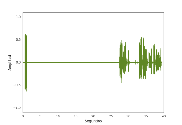
These arrays can be very large depending on the audio file's sample rate, and quite noisy too, especially when trying to identify silences. There may be short spikes in amplitude in an otherwise "silent" section, and in general, there is no true silence. Most silences are just low amplitude but not exactly 0.

In the example below you can see that what a person might consider silence has a few bits of very quiet sound scattered throughout.

Silences aren't exactly silent

There is also "noise" in the non-silent parts; that is, the signal can fluctuate quite suddenly, which can make analysis unwieldy.

To address these concerns, our preprocessing mostly consisted of:

  • Reducing the sample rate a bit so the arrays weren't so large, since the features we looked at don't need the precision of a higher sample rate.
  • Applying a smoothing function to deal with intermittent spikes in amplitude.
  • Zeroing out any amplitudes below 0.015 (i.e. we considered any amplitude under 0.015 to be silence).

Since we had about 20,000 labeled examples to process, we used joblib to parallelize the process, which improved speeds considerably.

The preprocessing scripts are available here.

Feature engineering

Typically, the main challenge in a machine learning problem is that of feature engineering - how do we take the raw audio data and represent it in a way that best suits the learning algorithm?

Audio files can be easily visualized, so our approach benefited from our own visual systems - we looked at a few examples from the voicemail and non-voicemail groups to see if any patterns jumped out immediately. Perhaps the clearest two patterns were the rings and the silence:

  • A voicemail file will also have a greater proportion of silence than sound. For this, we looked at the images generated from the audio and calculated the percentage of white pixels (representing silence) in the image.
  • A voicemail file will have several distinct rings, and the end of the file comes soon after the last ring. The intuition here is that no one picks up during a voicemail - hence many rings - and no one stays on the line much longer after the phone stops ringing. So we consider both the number of rings and the time from the last ring to the end of the file.

Ring analysis

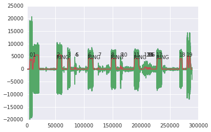
Identifying the rings is a challenge in itself - we developed a few heuristics which seem to work fairly well. You can see our complete analysis here, but the general idea is that we:

  • Identify non-silent parts, separated by silences
  • Check the length of the silence that precedes the non-silent part, if it is too short or too long, it is not a ring
  • Check the difference between maximum and minimum amplitudes of the non-silent part; it should be small if it's a ring

The example below shows the original audio waveform in green and the smoothed one in red. You can see that the rings are preceded by silences of a roughly equivalent length and that they look more like plateaus (flat-ish on the top). Another way of saying this is that rings have low variance in their amplitude. In contrast, the non-ring signal towards the end has much sharper peaks and vary a lot more in amplitude.

Automatic ring detection

Other features

We also considered a few other features:

  • Variance: voicemails have greater variance, since there is lots of silence punctuated by high-amplitude rings and not much in between.
  • Length: voicemails tend to be shorter since people hang up after a few rings.
  • Max amplitude: under the assumption that human speech is louder than the rings
  • Mean silence length: under the assumption that when people talk, there are only short silences (if any)

However, after some experimentation, the proportion of silence and the ring-based features performed the best.

Selecting, training, and evaluating the model

With the features in hand, the rest of the task is straightforward: it is a simple binary classification problem. An audio file is either a voicemail or not. We had several models to choose from; we tried logistic regression, random forest, and support vector machines since they are well-worn approaches that tend to perform well.

We first scaled the training data and then the testing data in the same way and computed cross validation scores for each model:

LogisticRegression
    roc_auc: 0.96 (+/- 0.02)
    average_precision: 0.94 (+/- 0.03)
    recall: 0.90 (+/- 0.04)
    f1: 0.88 (+/- 0.03)
RandomForestClassifier
    roc_auc: 0.96 (+/- 0.02)
    average_precision: 0.95 (+/- 0.02)
    recall: 0.89 (+/- 0.04)
    f1: 0.90 (+/- 0.03)
SVC
    roc_auc: 0.96 (+/- 0.02)
    average_precision: 0.94 (+/- 0.03)
    recall: 0.91 (+/- 0.04)
    f1: 0.90 (+/- 0.02)

We were curious what features were good predictors, so we looked at the relative importances of the features for both logistic regression:

[('length', -3.814302896584862),
 ('last_ring_to_end', 0.0056240364270560934),
('percent_silence', -0.67390678402142834),
('ring_count', 0.48483923341906693),
('white_proportion', 2.3131580570928114)]

And for the random forest classifier:

[('length', 0.30593363755717351),
 ('last_ring_to_end', 0.33353202776482688),
 ('percent_silence', 0.15206534339705702),
 ('ring_count', 0.0086084243372190443),
 ('white_proportion', 0.19986056694372359)]

Each of the models perform about the same, so we combined them all with a bagging approach (though in the notebook above we forgot to train each model on a different training subset, which may have helped performance), where we selected the label with the majority vote from the models.

Classification

We tried two variations on classifying the audio files, differing in where we set the probability cutoff for classifying a file as uninteresting or not.

in the balanced classification, we set the probability threshold to 0.5, so any audio file that has ≥ 0.5 of being uninteresting is classified as uninteresting. This approach labeled 8,069 files as discardable.
in the unbalanced classification, we set the threshold to the much stricter 0.9, so an audio file must have ≥ 0.9 chance of being uninteresting to be discarded. This approach labeled 5,785 files as discardable.

You can see the Jupyter notebook where we conducted the classification here.

Validation

We have also created a validation Jupyter notebook where we can cherry pick random results from our classified test set and verify the correctness ourselves by listening to the audio file and viewing its image.

The validation code is available here.

Summary

Even though using machine learning to classify audio is noisy and far from perfect, it can be useful making a problem more manageable. In our case, our solution narrowed the pool of audio files to only those that seem to be more interesting, reducing the time and resources needed to find the good stuff. We could always double check some of the discarded ones if there’s time to do that.


broca

07.31.2015
etc

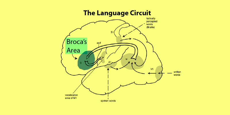
Broca's Area

At this year's OpenNews Code Convening, Alex Spangher of the New York Times and I worked on broca, which is a Python library for rapidly experimenting with new NLP approaches.

Conventional NLP methods - bag-of-words vector space representations of documents, for example - generally work well, but sometimes not well enough, or worse yet, not well at all. At that point, you might want to try out a lot of different methods that aren't available in popular NLP libraries.

Prior to the Code Convening, broca was little more than a hodgepodge of algorithms I'd implemented for various projects. During the Convening, we restructured the library, added some examples and tests, and implemented in the key piece of broca: pipelines.

Pipelines

The core of broca is organized around pipes, which take some input and produce some output, which are then chained into pipelines.

Pipes represent different stages of an NLP process - for instance, your first stage may involve preprocessing or cleaning up the document, the next may be vectorizing it, and so on.

In broca, this would look like:

from broca.pipeline import Pipeline
from broca.preprocess import Cleaner
from broca.vectorize import BoW

docs = [
    # ...
    # some string documents
    # ...
]

pipeline = Pipeline(
        Cleaner(),
        BoW()
)

vectors = pipeline(docs)

Since a key part of broca is rapid prototyping, it makes it very easy to simultaneously try different pipelines which may vary in only a few components:

from broca.vectorize import DCS

pipeline = Pipeline(
        Cleaner(),
        [BoW(), DCS()]
)

This would produce a multi-pipeline consisting of two pipelines: one which vectorizes using BoW, the other using DCS.

Multi-pipelines often have shared components. In the example above, Cleaner() is in both pipelines. To avoid redundant processing, a key part of broca's pipelines is that the output for each pipe is "frozen" to disk.

These frozen outputs are identified by a hash derived from the input data and other factors. If frozen output exists for a pipe and its input, that frozen output is "defrosted" and returned, saving unnecessary processing time.

broca's Cryo

This way, you can tweak different components of the pipeline without worrying about needing to re-compute a lot of data. Only the parts that have changed will be re-computed.

Included pipes

broca includes a few pipes:

  • broca.tokenize includes various tokenization methods, using lemmas and a few different keyword extractors.
  • broca.vectorize includes a traditional bag-of-words vectorizer, an implementation of "dismabiguated core semantics", and Doc2Vec.
  • broca.preprocess includes common preprocessors - cleaning punctuation, HTML, and a few others.

Other tools

Not everything in broca is a pipe. Also included are:

  • broca.similarity includes similarity methods for terms and documents.
  • broca.distance includes string distance methods (this may be renamed later).
  • broca.knowledge includes some tools for dealing with external knowledge sources (e.g. other corpora or Wikipedia).

Though at some point these may also become pipes.

Give us your pipes!

We made it really easy to implement your own pipes. Just inherit from the Pipe class, specify the class's input and output types, and implement the __call__ method (that's what's called for each pipe).

For example:

from broca.pipeline import Pipe

class MyPipe(Pipe):
    input = Pipe.type.docs
    output = Pipe.type.vecs

    def __init__(self, some_param):
        self.some_param = some_param

    def __call__(self, docs):
        # do something with docs to get vectors
        vecs = make_vecs_func(docs, self.some_param)
        return vecs

We hope that others will implement their own pipes and submit them as pull requests - it would be great if broca becomes a repository of sundry NLP methods which makes it super easy to quickly try a battery of techniques on a problem.

broca is available on GitHub and also via pip:

pip install broca

Fellowship Status Update

07.29.2015
etc

AI?

I've long been fascinated with the potential for technology to liberate people from things people would rather not be doing. This relationship between human and machine almost invariably manifests in the context of production processes - making this procedure a bit more efficient here, streamlining this process a bit there.

But what about social processes? A hallmark of the internet today is the utter ugliness that's possible of people; a seemingly inescapable blemish on the grand visions of the internet's potential for social transformation. And the internet's opening of the floodgates has had the expected effect of information everywhere, though perhaps in volumes greater than anyone anticipated.

Here we are, trying to engage little tyrants at considerable emotional expense. Here we are, futilely chipping away at the info-deluge we're suspended in. Here we are, both these things gradually chipping away at us. Things people would rather not be doing.

Blocker

Prior to my fellowship, these kinds of inquiries had to be relegated to off-hours skunkworks. The fellowship has given me the rare privilege of autonomy, both financial and temporal, and the resources, especially of the human kind, with which I can actually explore these questions as my job.

With the Coral Project, I'm researching what makes digital communities tick, surveying the problems with which they grapple, and learning about how different groups are approaching them - from video games to journalism to social networks both in the mainstream and the fringes (you can read my notes here). Soon we'll be building software to address these issues.

For my own projects I'm working on automatic summarization of comments sections, a service that keeps up with news when you can't, a reputation system for new social network, and all the auxiliary tools these kinds of projects tend to spawn, laying the groundwork for work I hope to continue long after the fellowship. I've been toying with the idea of simulating social networks to provide testing grounds for new automated community management tools. The best part is that it's up to me whether or not I pursue it.

A huge part of the fellowship is learning, which is something I love but have had to carve out my own time for. Here, it's part of the package. I've had ample opportunity to really dig into the sprawling landscape of machine learning and AI (my in-progress notes are here), something I've long wanted to do but never had the space for.

The applications for the 2016 fellowship are open, and I encourage you to apply. Rub shoulders with fantastic and talented folks from a variety of backgrounds. Pursue the questions that conventional employment prohibits you from. Explore topics and skills you've never had time for. It's really what you make of it. At the very least, it's a unique opportunity to be deliberate about where your work takes you.

The halfway mark of my OpenNews fellowship has just about passed. I knew from the start the time would pass by quickly, but I hadn't considered how much could happen in this short a time. There are only about 5 months left - the fellowship does end, but, fortunately, the work it inaugurates doesn't have to.


Geiger (Intro/Update)

07.27.2015
etc

A couple months ago I thought it would be interesting to see if a summary could be generated for a comment section. As a comment section grows, the comments become more repetitive as more people pile into make the same point. It also seems that some natural clustering forms as some commenters focus on particular aspects of an article or topic.

When there are hundreds to thousands of comments, there is little to be gained by reading all of them. However, it may be useful to quantify how much support certain opinions have, or what is most salient about a particular topic. What if there we had some automated means of presenting us such insight? For example, for an article about a new coal industry regulation: 27 comments are focused on how this regulation affects jobs, 39 are arguing about the environmental impacts, 6 are mentioning the meaning of this regulation in an international context, etc.

Having such insight can serve a number of purposes:

  • Provide a quick understanding of the salient points for readers of an article
  • Direct focus for future articles on the topic
  • Give a quick view into how people are responding to an article
  • Provide fodder for follow-up pieces on how people are responding
  • Surface entry points for other readers into the conversation

Geiger is still very much a work in progress and has led to a lot of experimentation, some of which worked ok, some of which didn't work at all, but so far nothing has worked as well as I'd like.

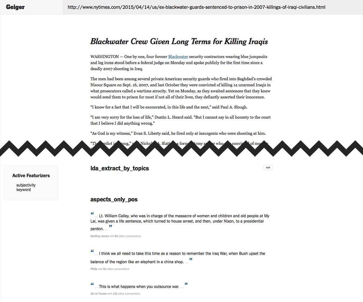
Below is a screenshot from an early prototype of Geiger which allowed me to try a battery of common techniques (TF-IDF bag of words with DBSCAN, K-Means, HAC, and LDA) and compare their results on any New York Times article with comments.

An early Geiger prototype

None of those led to particularly promising results, but a few alternatives were available.

Aspect summarization

This problem of clustering-to-summarize comments is similar to aspect summarization, which is more closely associated with ratings and reviews. For instance, you may have seen how Yelp's business pages have a few sentences selected at the top, with some term (the "aspect") highlighted, and then the number of reviewers that mentioned this term. That's aspect summarization - the aggregate reviews are being summarized by highlighting aspects which are mentioned the most.

Yelp's aspect summarization

Sometimes aspect summarization includes an additional layer of sentiment analysis, so that instead of just quantifying the number of people talking about an aspect, whether they are talking positively or negatively can also be surfaced (Yelp isn't doing this, however).

The process of aspect summarization can be broken down into three steps:

  1. Identify aspects
  2. Group documents by aspect
  3. Rank aspect groups

To identify aspects I used a few keyword extraction approaches (PoS tagging for noun phrases, named entity recognition, and other methods like Rapid Automatic Keyword Extraction) and then learned phrases by looking at keyword co-occurrences. If two keywords are adjacent (or separated by only a conjunction or hyphen) in at least 80% in the documents where they are present, we consider it a key phrase.

This simple co-occurrence approach is surprisingly effective. Here are some phrases learned on a set of comments for the coal industry regulation article:

'carbon tax', 'green energy', 'sun and wind', 'clean coal', 'air and water', 'high level', 'slow climate', 'middle class', 'signature environmental', 'mitch mcconnell', 'poor people', 'coal industry', 'true cost', 'clerical error', 'coal miner', 'representative democracy', 'co2 emission', 'power source', 'clean air', 'future generation', 'blah blah', 'ice age', 'planet earth', 'climate change', 'energy industry', 'critical thinking', 'particulate matter', 'coal mining', 'corporate interest', 'solar and wind', 'air act', 'acid rain', 'carbon dioxide', 'heavy metal', 'obama administration', 'monied interest', 'greenhouse gas', 'human specie', 'president obama', 'long term', 'political decision', 'big coal', 'coal and natural', 'al gore', 'bottom line', 'power generation', 'wind and solar', 'nuclear plant', 'global warming', 'human race', 'supreme court', 'environmental achievement', 'renewable source', 'coal ash', 'legal battle', 'united state', 'wind power', 'epa regulation', 'economic cost', 'federal government', 'state government', 'natural gas', 'west virginia', 'nuclear power', 'radioactive waste', 'battle begin', 'coal fire', 'energy source', 'common good', 'renewable energy', 'coal burning', 'nuclear energy', 'big tobacco', 'carbon footprint', 'red state', 'sea ice', 'peabody coal', 'tobacco industry', 'american citizen', 'fossil fuel', 'fuel industry', 'climate scientist', 'carbon credit', 'power plant', 'republican president', 'electricity cost'

Some additional processing steps were performed, such as removing keywords that were totally subsumed by key phrases; that is, keywords which only ever appear as part of a key phrase. Keywords were also stemmed and merged, e.g. "polluter", "pollute", "pollutant", "pollution" are grouped as a single aspect.

Grouping documents by aspects is straightforward (just look at overlaps). For this task I treated individual sentences as the documents, much like Yelp does.

Ranking them is a bit trickier. I used a combination of token length (assuming that phrases are more interesting than single keywords), support (number of sentences which mention the aspect), and IDF weighting of the aspect. The latter is useful because, for instance, we expect many comments will mention the "coal industry" if the article is about the coal industry, rendering it uninformative.

Although you get a bit of insight into what commenters are discussing, the results of this approach aren't very interesting. We don't really get any summary of what people are saying about an aspect. This is problematic when commenters are talking about an aspect in different ways. For instance, many commenters are talking about "climate change", but some ask whether or not the proposed regulation would be effective in mitigating it, whereas others debate whether or not climate change is a legitimate concern.

Finally, one problem here, which is consistent across all methods, is that this method is ignorant of synonymy - it cannot recognize when two words which look different mean essentially the same thing. For instance, colloquially people use "climate change" and "global warming" interchangeably, but here they are treated as two different aspects. This is a consequence of text similarity approaches which rely on matching the surface form of words - that is, which only look at exact term overlap.

This is especially challenging when dealing with short text documents, which I explain in greater length here.

Word2Vec word embeddings

There has been a lot of excitement around neural networks, and rightly so - their ability to learn representations is very useful. Word2Vec is capable of learning vector representations of words ("word embeddings") which allow us to capture some degree of semantic quality in vector space. For example, we could say that two words are semantically similar if their word embeddings are close to each other in vector space.

I loaded up Google's pre-trained Word2Vec model (trained on 100 billion words from a Google News dataset) and tested it out a bit. It seemed promising:

w2v.similarity('climate_change', 'global_warming')
>>> 0.88960381786226284

I made some attempts at approaches which leaned on this Word2Vec similarity of terms rather than their exact overlap - when comparing two documents A and B, each term from A is matched to is maximally-similar term in B and vice versa. Then the documents' similarity score is computed from these pairs' similarity values, weighted by their average IDF.

A problem with using Word2Vec word embeddings is that they are not really meant to quantify synonymy. Words that have embeddings close together do not necessarily mean similar things, all that it means is that they are exchangeable in some way. For example:

w2v.similarity('good', 'bad')
>>> 0.71900512146338569

The terms "good" and "bad" are definitely not synonyms, but they serve the same function (indicating quality or moral judgement) and so we expect to find them in similar contexts.

Because of this, Word2Vec ends up introducing more noise on occasion.

Measuring salience

Another angle I spent some time on was coming up with some better way of computing term "salience" - how interesting a term is. IDF is a good place to start, since a reasonable definition of a salient term is one that doesn't appear in every document, nor does it only appear in one or two documents. We want something more in the middle, since that indicates a term that commenters are congregating around.

Thus middle IDF values should be weighted higher than those closer to 0 or 1 (assuming these values are normalized to ¦[0,1]¦). To capture this, I put terms' IDF values through a Gaussian function with its peak at ¦x=0.5¦ and called the resulting value the term's "salience". Then, using the Word2Vec approach above, maximal pairs' similarity scores are weighted by their average salience instead of their average IDF.

The results of this technique look less noisy than before, but there is still ample room for improvement.

Challenges

Working through a variety of approaches has helped clarify what the main difficulties of the problem are:

  • Short texts lack a lot of helpful context
  • Recognizing synonymy is tricky
  • Noise - some terms aren't very interesting given the article or what other people are saying

What's next

More recently I have been trying a new clustering approach (hscluster) and exploring ways of better measuring short text similarity. I'm also going to take a deeper look into topic modeling methods, which I don't have a good grasp on yet but seem promising.

<< >>