Specifically for Linux. I'm using Ubuntu 22.04 and Unity 2021.3.22f1, with nvim-lspconfig.

This was a pretty heinous setup process, so I'm documenting this here to help others who want something similar. The actual setup process isn't too bad, but figuring out all the individual steps was difficult. I came across a few guides but some were out of date, or were geared towards Windows, or just didn't work for me.

I should also caveat that I'm writing this shortly after I got this setup working, so I may run into other issues with it once I start developing with it more. For example, there might be issues with new files. If I run into those problems and manage to solve them I'll update this post.

Requirements:

• omnisharp-roslyn, I'm using v1.39.6.
• mono; but crucially not the one from the default package repos. You need to use their official repo; then install: apt install mono-devel mono-complete.
  • The default Ubuntu package repo version doesn't include MSBuild so unless you use the official mono repo you'll get errors like "Could not locate MSBuild instance to register with OmniSharp." when running omnisharp-roslyn.

The process:

1. Download a release of omnisharp-roslyn (as mentioned above, I'm using v1.39.6). Extract it somewhere—for me, this was /opt/omnisharp-roslyn. The run file in that directory is what will start the LSP server.
2. Configure nvim. For me this all goes in ~/.vim/plugin/nvim-lsp.vim, but you can change that to match your own preference. I'm including the whole file but the key parts are what follows -- Omnisharp/C#/Unity. You must specify the path to the omnisharp-roslyn run script.

lua << EOF
local nvim_lsp = require('lspconfig')

-- Use an on_attach function to only map the following keys
-- after the language server attaches to the current buffer
local on_attach = function(client, bufnr)
  local function buf_set_keymap(...) vim.api.nvim_buf_set_keymap(bufnr, ...) end
  local function buf_set_option(...) vim.api.nvim_buf_set_option(bufnr, ...) end

  -- Omnicompletion
  buf_set_option('omnifunc', 'v:lua.vim.lsp.omnifunc')

  local opts = { noremap=true, silent=true }
  buf_set_keymap('n', 'gD', '<cmd>lua vim.lsp.buf.declaration()<CR>', opts)
  buf_set_keymap('n', 'gd', '<cmd>lua vim.lsp.buf.definition()<CR>', opts)
  buf_set_keymap('n', 'gi', '<cmd>lua vim.lsp.buf.implementation()<CR>', opts)
  buf_set_keymap('n', 'K', '<cmd>lua vim.lsp.buf.hover()<CR>', opts)
  buf_set_keymap('n', '<C-k>', '<cmd>lua vim.lsp.buf.signature_help()<CR>', opts)
  buf_set_keymap('n', '[d', '<cmd>lua vim.diagnostic.goto_prev()<CR>', opts)
  buf_set_keymap('n', ']d', '<cmd>lua vim.diagnostic.goto_next()<CR>', opts)
  buf_set_keymap('n', 'gR', '<cmd>lua vim.lsp.buf.references()<CR>', opts)
end

-- Omnisharp/C#/Unity
local pid = vim.fn.getpid()
local omnisharp_bin = "/opt/omnisharp-roslyn/run"
require'lspconfig'.omnisharp.setup{
    on_attach = on_attach,
    flags = {
      debounce_text_changes = 150,
    },
    cmd = { omnisharp_bin, "--languageserver" , "--hostPID", tostring(pid) };
}
EOF

3. Then we need to generate the .sln and .csproj files for our Unity project. There are two ways to do this:

   • Almost every other guide to this setup says you need to install Visual Studio Code to do this. This then requires that you go into your Unity project, go to Edit > Preferences > External Tools, then set Visual Studio Code to be your External Script Editor. Finally, check all the boxes for Generate .csproj files for:, then press Regenerate project files. This will work, and it's what I tried first.
   • The alternative, which I found here, is to run /opt/Unity/2021.3.22f1/Editor/Unity -batchmode -nographics -logFile - -executeMethod UnityEditor.SyncVS.SyncSolution -projectPath . -quit in your project root folder (note that /opt/Unity/2021.3.22f1/Editor/Unity is just where I installed the Unity Editor, so change that to point to your location). This will also work, and appears to work without installing VSCode. The only annoying bit is that a project can only be opened by one instance of the editor at a time, so this won't work if you already have your project open. Perhaps there's a way to call it from within Unity?

4. Finally, one issue I had was that for some reason Assembly-CSharp.csproj wasn't generated. This led to the Unity framework not being picked up by omnisharp, with errors like "The type or namespace name 'UnityEngine' could not be found". This solved itself by creating a new C# file, e.g. Assets/Foo.cs and then refreshing the project files in the Unity Editor (which I guess causes Unity to compile the scripts and then generate this missing file). No idea if this is necessary though.

Lastly, the LSP server is slow to start up on my machine. Something like 30 seconds. For Rust and TypeScript development I use this plugin, which gives me progress on those LSP servers' startups, but unfortunately it doesn't yet work for omnisharp.

NB: Just a couple debugging tips if this doesn't totally work for you: :LspInfo and :LspLog from within nvim can help you figure out what might be going wrong.

For the transit demand model for the PolicySpace project (see previously) we needed to be able to ingest GTFS (General Transit Feed Specification) data and use it to generate public transit routes. That is, given a start and an end stop, what's the quickest route using only public transit? Ideally we minimize both travel time and number of transfers, or strike some balance between the two.

I found an existing implementation here, based off of the papers Trip-Based Public Transit Routing (Sascha Witt, 2015) and Trip-Based Public Transit Routing Using Condensed Search Trees (Sascha Witt, 2016). The routing worked fine, but processing the Belo Horizonte GTFS data (630 routes with 9,428 stops, including buses and metro) took over 12 hours. The routing itself did not seem to have a significant speed gain from this pre-processing (unfortunately I don't have specific numbers on hand).

Instead I spent the past few days implementing my own public transit routing algorithm. It's a first attempt, and so it's naive/not heavily optimized, but so far seems to work alright. The goals were to significantly reduce pre-processing time, have a relatively low memory footprint, and quickly produce routes.

First, it's worth explaining a bit about how GTFS data is structured and the terminology it uses.

Public transit has a few components:

• stops: same as the colloquial usage; a 🚏stop is somewhere a bus, train, etc stops to pick up and drop off, described with an id and a latitude and longitude.
• trips: a 🚌trip is a sequence of stops associated with a set of arrival and departure times. For example, trip 🚌A goes through stop 🚏X at 12:00, then stop 🚏Y at 13:00, then stop 🚏Z at 14:00. Trip 🚌B goes through stop 🚏X at 13:00, then stop 🚏Y at 14:00, then stop 🚏Z at 15:00. Even though they have the same stop sequence (🚏X->🚏Y->🚏Z), they arrive/depart from each stop at different times, so they are distinct trips.
• route: a route is a collection of trips. A route's trips do not necessarily mean they share the exact same sequence of stops. For example, a route may have a trip that goes 🚏X->🚏Y->🚏Z and another trip that only goes 🚏X->🚏Y. (I didn't use this data and it's confusing because we're using the term "route" to describe something different. This is the last you'll see this particular usage in this post.)
• service: a service associates routes with days of operation (e.g. weekdays, weekends, off or alternative schedules on holidays, etc).

With these terms defined, we can define a public transit "route" more specifically as "a sequence of trips and their transfer stops". This is a bit more specific than how we describe routes conversationally, which is more like "take the Q line and transfer to the M at Foo Station". Instead, what we're after is more like "take the 12:42 train on the Q line, transfer to the 13:16 M at Foo Station".

GTFS data includes a few files (which are essentially CSVs but for whatever reason use the txt extension); the important ones here are:

• stop_times.txt: describes stop sequences for trips, as well as arrival and departure times for each trip's stops.
• stops.txt: describes stop latitudes and longitudes

We use some of the other data files as well, but those are more for juggling stop and trip ids and less core to the routing algorithm.

Transfer network: structure

The general approach is to generate a transfer network which describes at what stops are various trips linked together (i.e. where transfers can be made). The nodes of this network are described as (trip_id, stop_id) tuples. Note that not all stops of a trip will be nodes in the network; only those where transfers are made. Our resulting route only needs to return trips and where to transfer, not the individual stops within trips. That's something we can easily lookup later using the stop_times.txt data if needed.

The edges of this network can describe two different things:

• inter-trip edges: If an edge connects two nodes which share a trip_id, e.g. (🚌A, 🚏X)->(🚌A, 🚏Y), it indicates in the network structure that these nodes are along the same trip. Here the edge weight indicates travel time between stops 🚏X and 🚏Y for trip 🚌A.
• transfer edges: If an edge connects two nodes which don't share a trip_id, e.g. (🚌A, 🚏X)->(🚌B, 🚏X) it indicates a transfer between trips, e.g. transfer between trips 🚌A and 🚌B at stop 🚏X, and the edge weight indicates estimated transfer time.

We also need to distinguish between direct and indirect transfers:

• a direct transfer is one where the two connected trips share a stop. For example, (🚌A, 🚏X)->(🚌B, 🚏X) is a direct transfer because these trips both share the stop 🚏X.
• an indirect transfer is one where the two connected trips do not share a stop, but there is a reasonable footpath between the stops (i.e. you could walk between stops under some threshold transfer time limit, e.g. 5 minutes). For example (🚌A, 🚏X)->(🚌B, 🚏Y) where stop 🚏Y is around the corner from stop 🚏X. By introducing these additional edges, we potentially find shorter routes or routes where there normally wouldn't be one.

The transfer network is directed graph. This is due to the forward arrow of time. For example, trip 🚌A arrives at stop 🚏X at 12:10 and the 🚌B departs from stop 🚏X at 12:20, which indicates a valid transfer from trip 🚌A to 🚌B. However, I can't make the transfer in reverse; if I'm on trip 🚌B and arrive at 🚏X, trip 🚌A has potentially already departed from 🚏X. If the situation was that trip 🚌A lingers at 🚏X for long enough that the transfer does work in the reverse direction, we'd just have another edge (🚌B, 🚏Y)->(🚌A, 🚏X).

Transfer network: generation

The pre-processing step is almost entirely the generation of this transfer network. Once we have this network it's relatively easy to generate routes with Dijkstra's algorithm.

The generation process is broken into three parts:

1. Generate direct transfer edges
2. Generate indirect transfer edges
3. Generate inter-trip edges

Direct transfer edge generation

We can use the stop_times.txt file to identify direct transfers. We group rows according to stop_id and look at the trip_ids under each group. However, we can't just create edges between all these trips here; we have to filter in two ways:

1. down to valid transfers (those that obey the arrow of time). As noted before, a trip 🚌A can only transfer to a trip 🚌B at stop 🚏X if trip 🚌A arrives at 🚏X before trip 🚌B departs.
2. for each equivalent trip, select only the soonest to the incoming trip.

Expanding on 2): we assume that travellers want to make the soonest transfer possible from among a set of equivalent trips. Equivalent trips are those that share the same stop sequence, regardless of specific arrival/departure times. For example: a trip 🚌A with stops 🚏X->🚏Y->🚏Z and a trip 🚌B with stops 🚏X->🚏Y->🚏Z share the same stop sequence, and so are equivalent.

Say we have a trip 🚌C that also stops at stop 🚏X, arriving at 12:10. Trip 🚌A departs from 🚏X at 12:20 and trip 🚌B departs from 🚏X at 12:40. We only create the edge (🚌C, 🚏X)->(A, 🚏X) and not (🚌C, 🚏X)->(🚌B, 🚏X) because we assume no person will wait 20 extra minutes to take 🚌B when 🚌A goes along the exact same stops and departs sooner.

This assumption greatly reduces the number of edges in the network. With the Belo Horizonte data, this assumption cut edges by about 80%, roughly 18.5 million fewer edges!

Indirect transfer edge generation

To generate indirect transfers, we use the following process:

1. generate a spatial index (k-d tree) of all stops
2. for each stop 🚏X, find the n closest stops (neighbors)
   1. for each neighbor 🚏Y:
      1. compute estimated walking time between 🚏X and 🚏Y
      2. create edges between trips going through 🚏X and 🚏Y, sticking to the same constraints laid out for direct transfers (valid and soonest equivalent transfers)

The network edge count and processing time vary with n. Increasing n will, of course, increase edge count and processing time. I've been using n=3 but this will likely vary depending on the specifics of the public transit network you're looking at.

Generate inter-trip edges

Finally, we generate edges between nodes that share a trip. We link these nodes in their stop sequence order. For example, for a trip 🚌A with stop sequence 🚏X->🚏Y->🚏Z, where 🚏X and 🚏Z are both transfer stops, we should have a edge (🚌A,🚏X)->(🚌A,🚏Z). (🚌A,🚏Y) isn't in the graph because it isn't a transfer node.

Trip routing

Once the transfer network is ready we can leverage Dijkstra's algorithm to generate the trip routes. However, we want to accept any arbitrary start and end stops, whereas the nodes in our network only represent transfer stops. Not all stops are included. We use the following procedure to accommodate for this:

1. Given a starting stop 🚏s and departure time 🕒dt, find all trips 🚌T_s that go through 🚏s after 🕒dt.
2. Given a ending stop 🚏e, find all trips 🚌T_e that go through 🚏e after 🕒dt.
3. If there are trips in both 🚌T_s and 🚌T_e, that means there are trips from start to finish without any transfers. Return those and finish. Otherwise, continue.
4. For each potential starting trip 🚌t_s in 🚌T_s, find the transfer stop soonest after 🚏s in 🚌t_s (note that this could be 🚏s itself) to be an entry node into the transfer network. We'll denote these nodes as ⭕N_s. For example, if we have trip 🚌A with stop sequence 🚏X->🚏Y->🚏Z and 🚏X is our starting stop, but not a transfer stop (meaning it's not in our transfer network), and 🚏Y is a transfer stop, we get the node (🚌A, 🚏Y). If 🚏X is a transfer stop, then we just get (🚌A, 🚏X).
5. For each potential ending trip 🚌t_e in 🚌T_e, find the transfer stops closest to 🚏e in 🚌t_e (which could be 🚏e itself). We'll denote these nodes as ⭕N_e. This is just like step 4 except we go in reverse. For example, if we have trip 🚌A with the stop sequence 🚏X->🚏Y->🚏Z and 🚏Z is our starting stop but not a transfer stop, and 🚏Y is a transfer stop, then we get the node (🚌A, 🚏Y).
6. Create a dummy start node, ⭕START, and create edges from it to each node in ⭕N_s, where the edge weight is the travel time from stop 🚏s to that node.
7. Create a dummy end node, ⭕END, and create edges from each node in ⭕N_e to it, where the edge weight is the travel time from the node to stop 🚏e.
8. Use Dijkstra's algorithm to find the shortest weighted path from ⭕START to ⭕END. This path is our trip route.

Conclusion

On the Belo Horizonte data (630 routes with 9,428 stops) with n=3 for indirect transfer generation we get a graph of 239,667 nodes and 4,879,935 edges. I haven't yet figured out a way to further reduce this edge count.

The transfer network generation takes about 20 minutes on my ThinkPad X260. I'm not certain a direct comparison is appropriate, but this is significantly faster than the 12 hours the other implementation took. The actual route generation doesn't seem any faster or slower than the other implementation.

While the routing is fairly fast, it definitely could be faster, and is not fast enough for direct usage in PolicySpace. We won't be able to compute individual trip routes for every one of Brazil's ~209 million inhabitants, but we were never expecting to either. This trip routing feature will be used by some higher-level interface which will cache routes and batch compute more approximate routes between regions (called "transportation analysis zones" in the transit demand modeling literature) to cut down on processing time. We're still figuring out specifics.

Anyway, this is version 1 of this trip routing method — I'd appreciate any feedback and suggestions on how to improve the approach. I need to do more testing to get a better sense of the generated routes' quality.

The code for this implementation at time of writing is available here. There are a couple names different in the code than described here, e.g. the transfer network is called a "trip network", but the algorithm itself should be the same.

ProtonMail recently released their Linux beta for Bridge, which provides IMAP/SMTP access to the service. Prior to Bridge you could only access the service through the web interface, which is sort of clunky and requires you to, among other things, rely on their search, which is limited by the fact that they can't really index your emails - because you're paying them not to read the message bodies!

ProtonMail provides instructions for setting up the Bridge with common email applications like Thunderbird, but that's about it. So here's how to set it up with NeoMutt and OfflineIMAP for fetching our emails.

(My full email setup also includes the common Mutt companions NotMuch for better searching and urlscan for viewing URLs more easily in emails, in addition to some custom scripts, such as one for viewing HTML emails in a nice popover window and one for viewing MHT/MHTML emails (which are emails that contain inline attachments). It's too much to cover here, but if you want to poke around these scripts and my full email configs (at time of writing), see my dippindots.)

Installing NeoMutt and OfflineIMAP

These instructions are for Ubuntu 16.04, but I imagine they aren't much different for other distributions (yours might even have a package you can install).

Install dependencies:

sudo apt install -y xsltproc libidn11-dev libsasl2-dev libnotmuch-dev --no-install-recommends

Then grab the latest NeoMutt release, extract, and build:

./configure --disable-doc --ssl --sasl --notmuch
make
sudo make install

# so we can just access it via `mutt`
sudo ln -s /usr/bin/neomutt /usr/bin/mutt

Then install OfflineIMAP:

sudo pip install offlineimap

Running the Bridge

The Bridge can be run from the command line with the Desktop-Bridge program. By default this opens a GUI to setup your accounts, but you can also access a console interface with Desktop-Bridge --cli.

If you aren't already logged in you need to run the login command in this interface.

Configuring OfflineIMAP

First thing to do is configure OfflineIMAP to access our ProtonMail emails.

OfflineIMAP looks for a config at ~/.offlineimaprc. My config at time of writing is:

[general]
accounts = main


[Account main]
localrepository = main-local
remoterepository = main-remote

# full refresh, in min
autorefresh = 0.2

# quick refreshs between each full refresh
quick = 10

# update notmuch index after sync
postsynchook = notmuch new


[Repository main-local]
type = Maildir
localfolders = ~/.mail

# delete remote mails that were deleted locally
sync_deletes = yes


[Repository main-remote]
type = IMAP
remoteport = 1143
remotehost = 127.0.0.1
remoteuser = <YOUR EMAIL>
remotepass = <YOUR BRIDGE-SPECIFIC PASSWORD>
keepalive = 60
holdconnectionopen = yes

# delete local mails that were deleted on the remote server
expunge = yes

# sync only these folders
folderfilter = lambda foldername: foldername in ['INBOX', 'Archive', 'Sent']

# is broken, but connecting locally to bridge so should be ok
ssl = no

Basically this sets up an account arbitrarily called main which will store emails at ~/.mail in the Maildir format. It will only sync the INBOX, Archive, and Sent folders to/from ProtonMail (the folderfilter option). Emails deleted locally will also be deleted on ProtonMail (the sync_deletes option) and emails deleted on ProtonMail will be deleted locally (the expunge option).

After OfflineIMAP fetches new email, it will run the command defined for postsynchook, which in this case is is the notmuch command for updating its search index (notmuch new).

Important Bridge-related things to note:

• Bridge generates a Bridge-specific password for you to use, so use that here and not your actual ProtonMail password.
• Bridge's IMAP service runs at 127.0.0.1:1143 (normally IMAP runs on port 143 or 993 for SSL)
• Disable SSL because it was (at least when I set this up) not working with Bridge. But this seems like a non-issue because it's over a local connection anyways and the actual outgoing connection to ProtonMail is encrypted.

Then try running it using the offlineimap command.

Configuring NeoMutt

There is a lot to configure in NeoMutt, so I'll only cover what is necessary to get this setup working. If you're interested in seeing more, my NeoMutt config at time of writing is available here.

NeoMutt looks for a config at ~/.muttrc. To get it working with OfflineIMAP and to send emails with SMTP you need at least:

# "+" substitutes for `folder`
set mbox_type=Maildir
set folder=~/.mail/
set record=+Sent
set postponed=+Drafts
set trash=+Trash
set mail_check=2 # seconds

# smtp
source ~/docs/keys/mail
set smtp_url=smtp://$my_user:$my_pass@127.0.0.1:1025
set ssl_force_tls
set ssl_starttls

Where my ~/docs/keys/mail file has contents in the format:

set my_user=<YOUR EMAIL>
set my_pass=<YOUR BRIDGE-SPECIFIC PASSWORD>

Important Bridge-related notes:

• The SMTP port is 1025 (typically it's 587)
• See the previous note on Bridge-specific password

That should be all you need.

"Daemonizing" the Bridge

There currently is no way to daemonize the Bridge, but here's a workaround using tmux:

tmux new-session -d -s mail 'Desktop-Bridge --cli'

This just opens up a new tmux session and runs the Bridge inside of it.

I encountered an interesting challenge the other day while working on a transit demand model for the PolicySpace project (under Bernardo Furtado at the IPEA/Institute of Applied Economic Research).

We have bus data for Belo Horizonte, one of the largest cities in Brazil (and South America). Specifically, we have GTFS (General Transit Feed Specification) data with geographic coordinates of bus stops.

We also have a network of the city's roads, with data provided by OpenStreetMaps and accessed with the osmnx library. The library provides us with the geographic and UTM (Universal Transverse Mercator) projected coordinates for nodes as well as line geometries for most of the edges (edges which are just straight lines don't have geometries provided, but they can be inferred from the coordinates of their start and end nodes).

How do we meaningfully map these bus stops to our road network? The first instinct might be to associate them with their closest node, but many bus stops start somewhere along a road rather than at the start or end of one.

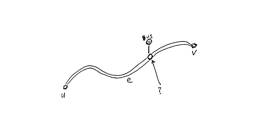
So we need to be able to find the closest point along a road for a given bus stop. This is trickier because whereas nodes can be treated as single points, roads potentially have winding geometries. A road which starts and ends far from a bus stop might nevertheless have a very close point to the bus stop somewhere along it. We want to accommodate these kinds of cases.

The first step is to find candidate edges that are close enough to the bus stop to be plausible roads for it. We have bounding boxes for each edge's geometry, so we can accomplish this search with a quadtree, using Pyqtree. A quadtree is a data structure that indexes 2D boxes and allows you to quickly find boxes which overlap a given query box. It's sort of like a kd-tree but can search boxes in addition to points.

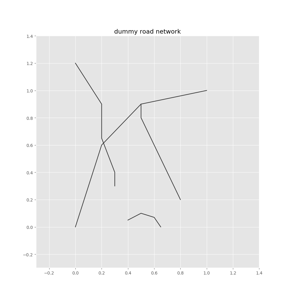
To demonstrate this process, I'll use a dummy road network consisting of a few paths:

bbox = (-0.3, -0.3, 1.4, 1.4)
paths = [
    [(0, 0), (0.2, 0.6), (0.5, 0.9), (1, 1)],
    [(0.8, 0.2), (0.5, 0.8), (0.5, 0.9)],
    [(0.4, 0.05), (0.5, 0.1), (0.6, 0.07), (0.65, 0)],
    [(0, 1.2), (0.2, 0.9), (0.2, 0.65), (0.3, 0.4), (0.3, 0.3)],
]

Which looks like:

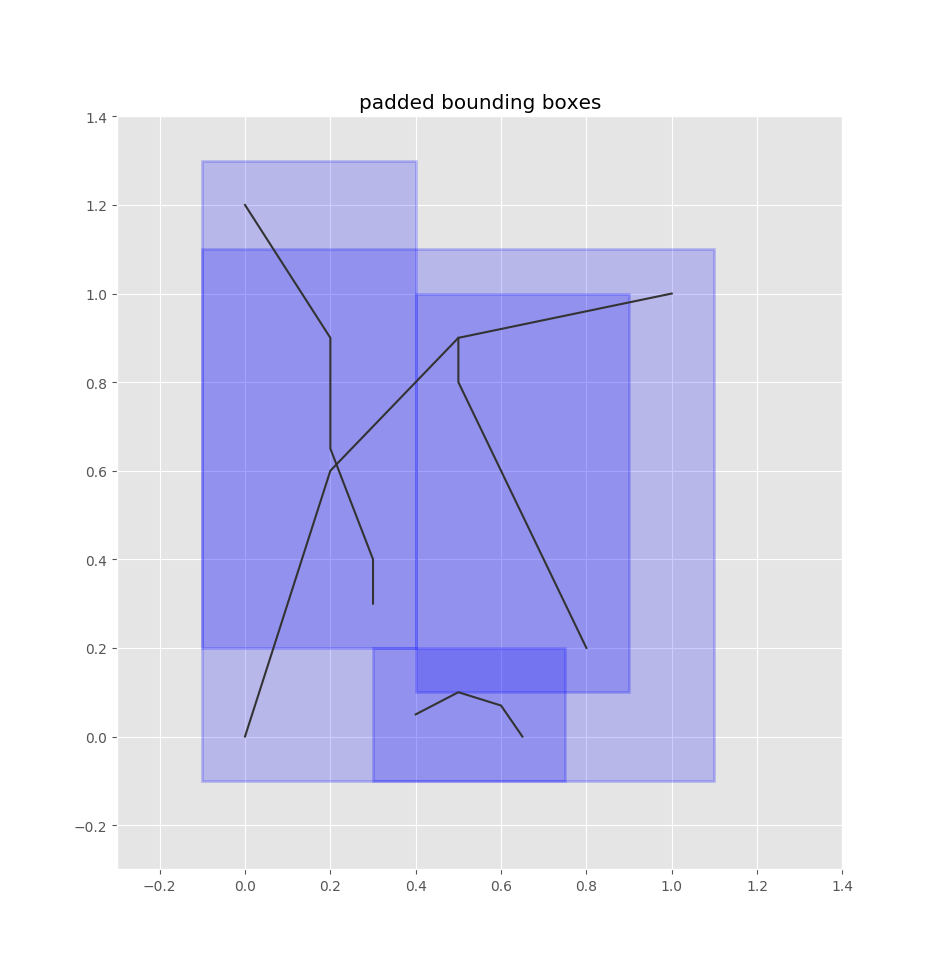
So we index all our edges' bounding boxes into this quadtree. We pad the bounding boxes by some configurable radius, since the bus stop is likely to be in the vicinity of an edge's borders.

from pyqtree import Index
from shapely import geometry

# box padding
radius = 0.1

# keep track of lines so we can
# recover them later
lines = []

# initialize the quadtree index
idx = Index(bbox)

# add edge bounding boxes to the index
for i, path in enumerate(paths):
    # create line geometry
    line = geometry.LineString(path)

    # bounding boxes, with padding
    x1, y1, x2, y2 = line.bounds
    bounds = x1-radius, y1-radius, x2+radius, y2+radius

    # add to quadtree
    idx.insert(i, bounds)

    # save the line for later use
    lines.append((line, bounds))

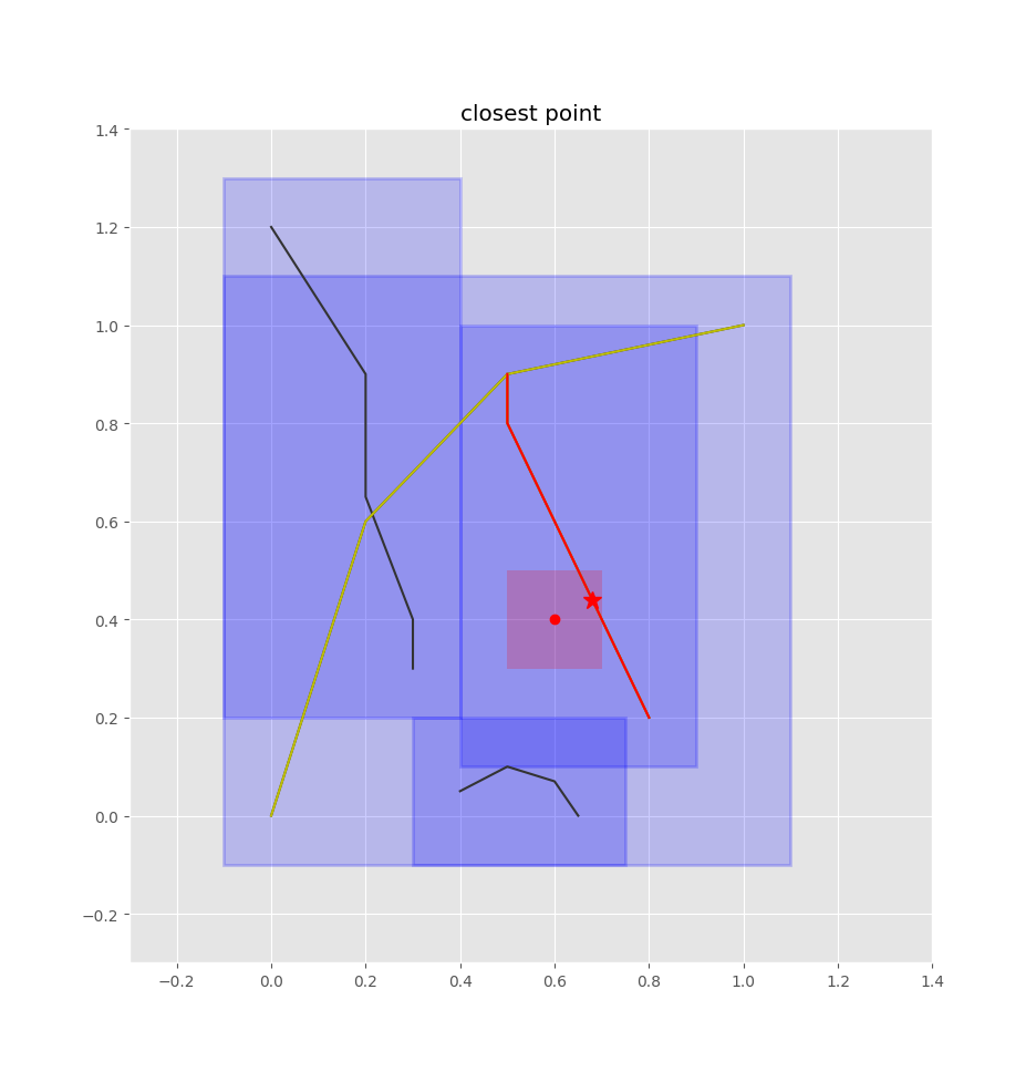
Here's what these bounding boxes look like for the demo network:

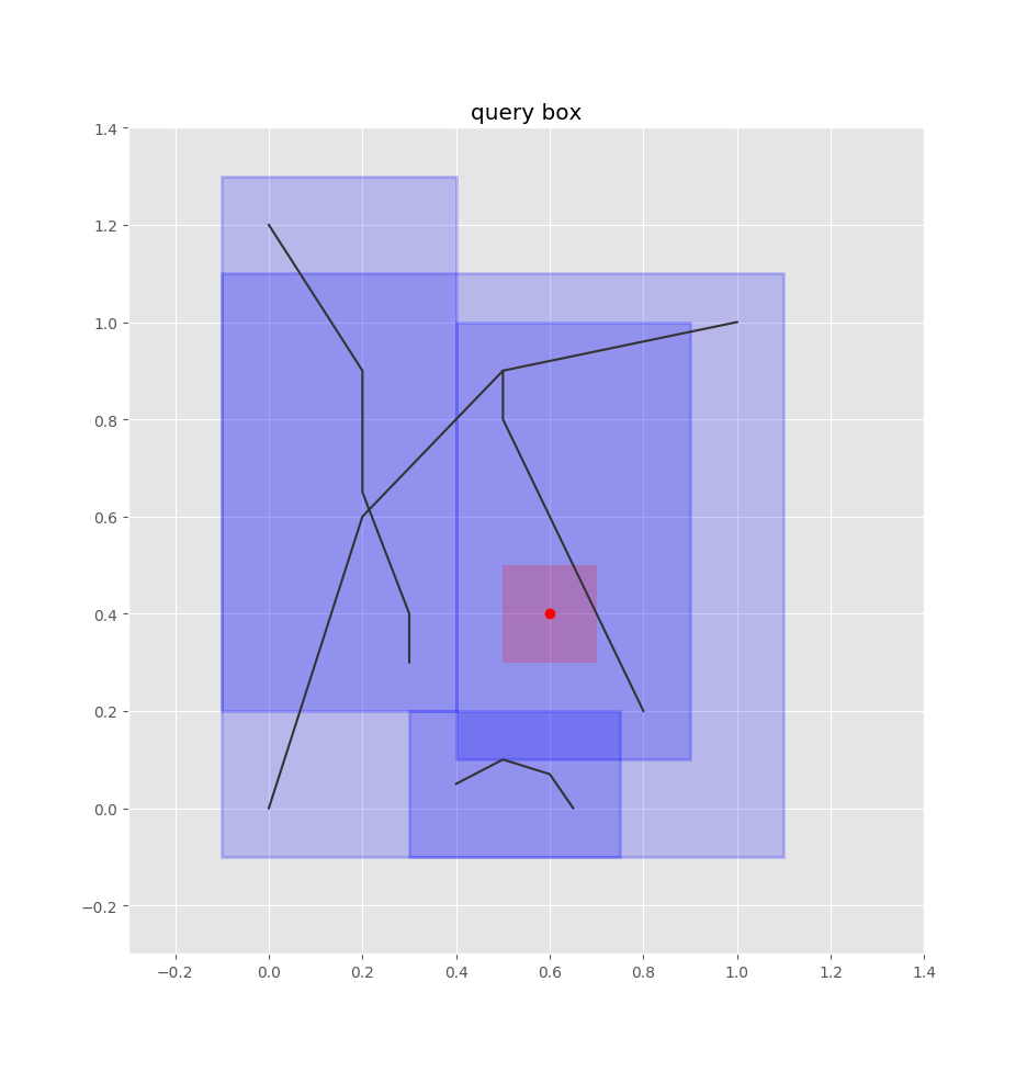
Let's say we have a bus stop at the following red point:

To find the closest edges using the quadtree, we treat this point as a box, adding some padding to it as well:

# query point
pt = geometry.Point(0.6, 0.4)

# query box
pt_bounds = pt.x-radius, pt.y-radius, pt.x+radius, pt.y+radius

Querying the quadtree is simple:

matches = idx.intersect(pt_bounds)

Now it's a matter of finding the closest edge. We're using shapely's geometry objects which have a lot of what we need built-in:

# find closest path
closest_path = min(matches, key=lambda i: lines[i][0].distance(pt))
closest_line = lines[closest_path][0]

Once we have the closest edge, we find the closest point on that edge by projecting the query point onto the edge. We don't want an absolute position, but rather how far the point is along the edge. That is, we want a value in [0,1] such that 0 is the start of the edge, 1 is the end of the edge, 0.5 is halfway along the edge, etc. shapely's normalized=True argument will take care of that for us.

p = closest_line.project(pt, normalized=True)

If we want the absolute point to, for example, plot it below, we can get it easily:

closest_pt = closest_line.interpolate(p, normalized=True)

Now we have mappings of bus stops to positions along edges, which we can leverage when computing trip routes for our transit demand model.

Yesterday I started working on a new game, tentatively titled "Trolley Problems: A Eulogy for Social Norms". This will be my second game with Three.js and Blender (though the first, The Founder, is still not totally finished) and I thought it'd be helpful to document this process.

The game isn't very far at this point. This video shows its current state:

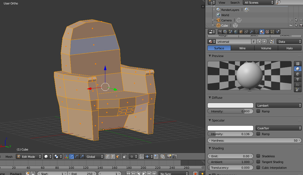
The basic process was: 1) create the chair model in Blender and 2) load the chair into Three.js.

Blender

I won't give a Blender modeling tutorial here (this was suggested as a good resource to start), but the theater chair model was quickly made by extruding a bunch from a cube.

A lot of the model's character comes out in the texturing. I like to keep textures really simple, just combinations of solid colors. The way I do it is with a single texture file that I gradually add to throughout a project. Each pixel is a color, so the texture is basically a palette.

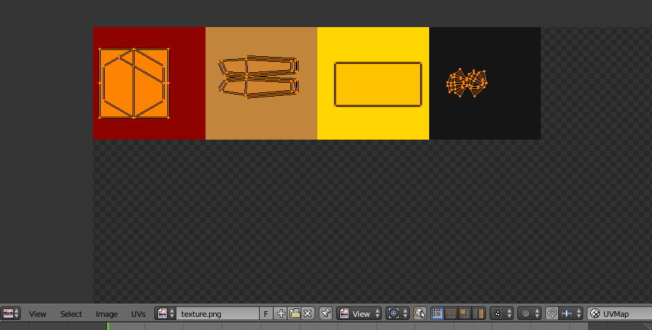
In Blender I just select the faces I want to have a particular color, use the default UV map unwrapping (while in Edit Mode, hit U and select Unwrap) and then in UV/Image Editor (with the texture file selected in the dropdown, see image below) I just drag the unwrapped faces onto the appropriate colors.

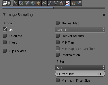
There is one thing you have to do to get this texture rendering properly. By default, Blender (like almost every other 3D program) will try to scale your textures.

In the texture properties window (select the red-and-white checker icon in the Properties window, see below), scroll down and expand the Image Sampling section. Uncheck MIP Map and Interpolation, then set Filter to Box (see below for the correct settings). This will stop Blender from trying to scale the texture and give you the nice solid color you want.

Here's a Blender render of the outcome:

Exporting to Three.js

One of the best things about Three.js is that there is a Blender-to-Three.js exporter. Installation is pretty straightforward (described in the repo here).

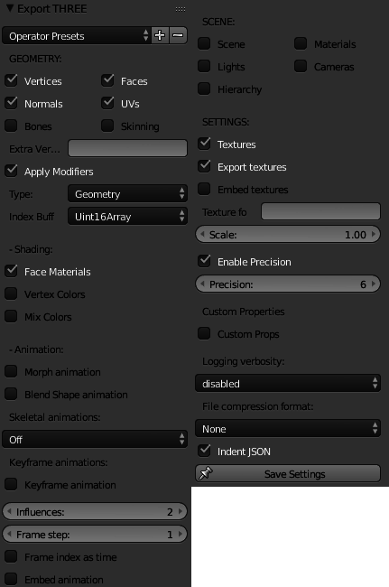
To export a Blender object to JSON, select your object (in Object Mode) and select from the menu File > Export > Three (.json).

The export options can be a bit finicky, depending on what you want to export the model for. For a basic static model like this chair the following settings should work fine:

That's all that Blender's needed for.

Three.js

This next section involves a bunch of code. I won't reproduce everything here (you can check out the repo to see the full working example) but I'll highlight the important parts.

Loading the model

Three.js provides a JSONLoader class which is what loads the exported Blender model. You could just use that and be done with it, but there are a few modifications I make to the loaded model to get it looking right.

const meshLoader = new THREE.JSONLoader();
meshLoader.load('assets/theater_chair.json', function(geometry, materials) {
    // you could just directly use the materials loaded from JSON,
    // but I like to make sure I'm using the proper material.
    // we extract the texture from the loaded material and pass it to
    // the MeshLambertMaterial here
    var texture  = materials[0].map,
        material = new THREE.MeshLambertMaterial({map: texture}),
        mesh = new THREE.Mesh(geometry, material);

    // material adjustments to get the right look
    material.shininess = 0;
    material.shading = THREE.FlatShading;

    // basically what we did with blender to prevent texture scaling
    material.map.generateMipmaps = false;
    material.map.magFilter = THREE.NearestFilter;
    material.map.minFilter = THREE.NearestFilter;

    // increase saturation/brightness
    material.emissiveIntensity = 1;
    material.emissive = {r: 0, g: 0, b: 0};
    material.color = {
        r: 2.5,
        g: 2.5,
        b: 2.5
    };

    mesh.position.set(0,5,0);
    scene.add(mesh);
});

The above code won't work until we create the scene. I like to bundle the scene-related stuff together into a Scene class:

class Scene {
    constructor(lightColor, groundColor, skyColor, fogColor, fogDistance) {
        this.camera = new THREE.PerspectiveCamera(75, window.innerWidth / window.innerHeight, 1, 1000);
        this.scene = new THREE.Scene();
        this.scene.fog = new THREE.Fog(fogColor, 0, fogDistance);
        var light = new THREE.HemisphereLight(lightColor, 0x777788, 0.75);
        light.position.set(0.5, 1, 0.75);
        this.scene.add(light);

        // setup floor
        var geometry = new THREE.PlaneGeometry(2000, 2000, 100, 100);
        geometry.rotateX(-Math.PI/2);
        var material = new THREE.MeshLambertMaterial({color: groundColor});
        var mesh = new THREE.Mesh(geometry, material);
        this.scene.add(mesh);

        this.renderer = new THREE.WebGLRenderer();
        this.renderer.setClearColor(skyColor);
        this.renderer.setPixelRatio(window.devicePixelRatio);
        this.renderer.setSize(window.innerWidth, window.innerHeight);
        document.body.appendChild(this.renderer.domElement);

        window.addEventListener('resize', this.onWindowResize.bind(this), false);
    }

    render() {
        requestAnimationFrame(this.render.bind(this));
        this.renderer.render(this.scene, this.camera);
    }

    add(mesh) {
        this.scene.add(mesh);
    }

    onWindowResize() {
        this.camera.aspect = window.innerWidth/window.innerHeight;
        this.camera.updateProjectionMatrix();
        this.renderer.setSize(window.innerWidth, window.innerHeight);
    }
}

It can be used like this:

var scene = new Scene();
scene.render();

And the previous code for loading the chair should place the chair into the scene.

First-person interaction

So far you won't be able to look or walk around the scene, so we need to add some first-person interaction. There are two components to this:

1. movement (when you press WASD or the arrow keys, you move forward/backwards/left/right)
2. looking around (when you move the mouse)

Movement

In the Scene class the onKeyDown and onKeyUp methods determine, based on what keys you press and release, which direction you should move in. The render method includes some additional code to check which directions you're supposed to be moving in and adds the appropriate velocity.

The velocity x value moves you right (positive) and negative (negative), the y value moves you up (positive) and down (negative), and the z value moves you forward (negative) and backwards (positive). It's important to note that the z value is negative in the forward direction because this confused me for a while.

We also keep track of how much time elapsed since the last frame (delta) so we scale the velocity appropriately (e.g. if the last frame update was 0.5s ago, you should move only half as far as you would if it had been 1s ago).

You'll notice that you can walk through objects which is probably not what you want...we'll add simple collision detection later to fix this.

Looking around

The key to looking around is the browser's pointer lock API. The pointer lock API allows you to capture your mouse cursor and its movement.

I'd never done this before, but the Three.js repo includes an example that shows the basic method. So I gutted that and moved the important bits into the Scene class. The full code is available here), but I'll explain some of it here.

In the Scene class the important method is setupPointerLock, which sets up the pointer lock event listeners. It is pretty straightforward, but basically: there's an instructions element that, when clicked on, locks the pointer and puts the game into fullscreen.

The onPointerLockChange method toggles the pointer lock controls, so that the controls are only listening when the pointer lock is engaged.

The meat of the actual pointer movement is handled in PointerLock.js. This is directly lifted from the Three.js example implementation. It's also pretty sparse; it adjusts the yaw and pitch of the camera according to how you move your mouse.

We have to properly initialize these controls though. In the Scene's constructor the following are added:

    // ...
    this.controls = new THREE.PointerLockControls(this.camera);
    this.scene.add(this.controls.getObject());
    // ...

Collision detection

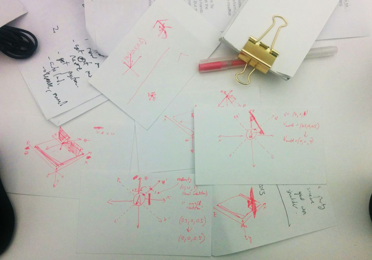
So the last bit here is to prevent the player from walking through stuff. I have a terrible intuition about 3D graphics so this took me way too long. Below are some of my scribbles from trying to understand the problem.

The basic approach is to use raycasting, which involves "casting" a "ray" out from a point in some direction. Then you can check if this ray intersects with any objects and how far away those objects are.

Below are an example of some rays. For example, the one going in front of the object points to (0,0,1). That sounds like it contradicts what I said earlier about the front of the object being in the negative-z direction...it doesn't quite. This will become important and confusing later.

The rays that I'm using are:

const RAYS = [
  new THREE.Vector3( 0,  0, -1), // back
  new THREE.Vector3( 1,  0, -1), // back-right
  new THREE.Vector3(-1,  0, -1), // back-left
  new THREE.Vector3( 0,  0,  1), // forward
  new THREE.Vector3( 1,  0,  1), // forward-right
  new THREE.Vector3(-1,  0,  1), // forward-left
  new THREE.Vector3( 1,  0,  0), // right
  new THREE.Vector3(-1,  0,  0), // left
  new THREE.Vector3( 0, -1,  0), // bottom
];

Note that the comments in the example on GitHub are incorrect (they have right and left switched...like I said, this was very confusing for me).

Every update we cast these rays and see if they intersect with any objects. We check if those objects are within some collision distance, and if they are, we zero out the velocity in that direction. So, for instance, if you're trying to move in the negative-z direction (forward) and there's an object in front of you, we have to set velocity.z = 0 to stop you moving in that direction.

That sounds pretty straightforward but there's one catch - the velocity is relative to where you're facing (i.e. the player's axis), e.g. if velocity.z is -1 that means you're moving in the direction you're looking at, which might not be the "true" world negative-z direction.

These rays, unlike velocity, are cast in directions relative to the world axis.

This might be clearer with an example.

Say you're facing in the positive-x direction (i.e. to the right). When you move forward (i.e. press W), velocity.z will be some negative value and velocity.x will be zero (we'll say your velocity is (0,0,-1)). This is because according to your orientation, "forward" is always negative-z, even though in the context of the world your "forward" is technically positive-x. Your positive-x (your right) is in the world's negative-z direction (see how this is confusing??).

Now let's say an object is in front of you. Because our raycasters work based on the world context, it will say there's an obstacle in the positive-x direction. We want to zero-out the velocity in that direction (so you're blocked from moving in that direction). However, we can't just zero-out velocity.x because that does not actually correspond to the direction you're moving in. In this particular example we need to zero-out velocity.z because, from your perspective, the obstacle is in front of you (negative-z direction), not to your right (positive-x direction).

The general approach I took (and I'm not sure if it's particularly robust, but it seems ok for now) is to take your ("local") velocity, translate it to the world context (i.e. from our example, a velocity of (0,0,-1) gets translated to (1,0,0)). Then I check the raycasters, apply the velocity zeroing-out to this transformed ("world") velocity (so if there is an obstacle in the positive-x direction, I zero out the x value to get a world velocity of (0,0,0)), then re-translate it back into the local velocity.

Ok, so here's how this ends up getting implemented.

First I add the following initialization code to the Scene's constructor:

    // ...
    this.height = 10;
    this.collidable = [];
    this.collisionDistance = 15;
    this.raycaster = new THREE.Raycaster(new THREE.Vector3(), new THREE.Vector3(0, -1, 0), 0, this.height);
    // ...

Whenever you add a mesh and the player shouldn't be able to walk through it, you need to add that mesh to this.collidable.

Then I add a detectCollisions method onto the Scene class:

detectCollisions() {
    // the quaternion describes the rotation of the player
    var quaternion = this.controls.getObject().quaternion,
        adjVel = this.velocity.clone();

    // don't forget to flip that z-axis so that forward becomes positive again
    adjVel.z *= -1;

    // we detect collisions about halfway up the player's height
    // if an object is positioned below or above this height (and is too small to cross it)
    // it will NOT be collided with
    var pos = this.controls.getObject().position.clone();
    pos.y -= this.height/2;

    // to get the world velocity, apply the _inverse_ of the player's rotation
    // effectively "undoing" it
    var worldVelocity = adjVel.applyQuaternion(quaternion.clone().inverse());

    // then, for each ray
    _.each(RAYS, (ray, i) => {
      // set the raycaster to start from the player and go in the direction of the ray
      this.raycaster.set(pos, ray);

      // check if we collide with anything
      var collisions = this.raycaster.intersectObjects(this.collidable);
      if (collisions.length > 0 && collisions[0].distance <= this.collisionDistance) {
        switch (i) {
          case 0:
            // console.log('object in true back');
            if (worldVelocity.z > 0) worldVelocity.z = 0;
            break;
          case 1:
            // console.log('object in true back-left');
            if (worldVelocity.z > 0) worldVelocity.z = 0;
            if (worldVelocity.x > 0) worldVelocity.x = 0;
            break;
          case 2:
            // console.log('object in true back-right');
            if (worldVelocity.z > 0) worldVelocity.z = 0;
            if (worldVelocity.x < 0) worldVelocity.x = 0;
            break;
          case 3:
            // console.log('object in true front');
            if (worldVelocity.z < 0) worldVelocity.z = 0;
            break;
          case 4:
            // console.log('object in true front-left');
            if (worldVelocity.z < 0) worldVelocity.z = 0;
            if (worldVelocity.x > 0) worldVelocity.x = 0;
            break;
          case 5:
            // console.log('object in true front-right');
            if (worldVelocity.z < 0) worldVelocity.z = 0;
            if (worldVelocity.x < 0) worldVelocity.x = 0;
            break;
          case 6:
            // console.log('object in true left');
            if (worldVelocity.x > 0) worldVelocity.x = 0;
            break;
          case 7:
            // console.log('object in true right');
            if (worldVelocity.x < 0) worldVelocity.x = 0;
            break;
          case 8:
            // console.log('object in true bottom');
            if (worldVelocity.y < 0) worldVelocity.y = 0;
            break;
        }
      }
    });

    // re-apply the player's rotation and re-flip the z-axis
    // so the velocity is relative to the player again
    this.velocity = worldVelocity.applyQuaternion(quaternion);
    this.velocity.z *= -1;
}

This is working for me so far. The code can probably be more concise and I suspect there's a much more direct route (involving matrix multiplication or something) to accomplish this. But I can wrap my head around this approach and it makes sense :)